Journals
Computed tomography texture feature stability dependence on the graylevel co-occurrence matrix discretization approach
A B S T R A C T
Purpose: To explore the effects of the discretization approach on the stability of the second-order computed tomography (CT) based textural features, derived from gray-level co-occurrence matrices (GLCMs).
Material and Methods: A Cathphan phantom was scanned seven times over three weeks. Four cylindrical regions (ROIs) were manually outlined for each scan. Two regions had fairly uniform density, while the other two were more heterogeneous. For each ROI four GLCMs were created – with 64 bins, with 32 bins, and with fixed bin widths of 1 and 4 HU. Eighteen commonly used radiomics features were calculated form the GLCMs, and their variabilities were compared among the four GLCM representations.
Results: The uniform ROIs had average standard deviation of the HUs of ~1.5%, while the heterogeneous ROIs had standard deviations greater than 4%. For the uniform ROIs the variability of the fixed number of bins GLCMs was on average lower than the variability for fixed bin width GLCMs. For the heterogeneous ROIs the situation was reversed. For the uniform ROIs the variability of the mean, variance, and energy decreased when the corresponding quantities were multiplied by the RIO volumes. Variabilities of the majority of the remaining features for those ROIs were also reduced when the features were normalized to the HU ranges or to the ROI volumes. For heterogeneous ROIs the mean, variance, energy, auto correlation, and correlation were weakly dependent on volume and range. The variability of fixed number of bins GLCMs exhibited strong dependence on the ROI range.
Conclusion: This study indicates that the GLCMs creation is affected differently depending on the homogeneity of the ROI. The fixed number of bins GLCMs produce fewer variable features for homogenous objects and vice-versa. Additionally, it was demonstrated that for realistic patient scenarios the use of fixed bin width GLCMs may be advantageous
K E Y W O R D S
quantitative, imaging, biomarker, stability, CT, GLCM
I N T R O D U C T I O N
In the last several years the field of quantitative medical imaging has rapidly developed. The field of the so called radiomics holds potential for improved cancer diagnoses and management [1-3]. Publications on quantitative imaging range from studies that utilize very few and basic features to studies that extract a large number of much more sophisticated quantities [1, 3-8]. Extraction of imaging features has been applied to almost all available imaging modalities – plain radiographs, computed tomography (CT), positron emission tomography (PET), magnetic resonance imaging (MRI), functional MRI, etc [3, 9-23]. The most widely used quantitative image measures include one-dimensional features such as tumor size, mean voxel (volume element) intensity, and intensity standard deviation, which are easy to understand and straightforward to obtain [24-26]. They were developed historically on the basis of clinician experience with cancer therapy and subsequent outcomes.
More recent medical imaging quantitative features are usually statistical-, model-, or transform-based [27]. They are more complex than the early quantitative measures and reflect variations in tumor morphology, heterogeneity, and texture [28]. Image texture in particular is defined as a spatial arrangement of the voxels comprising the tumors that allow the extraction of elaborate image properties and/or patterns. A textural feature is defined as a measure derived from a texture matrix.22 The texture matrices are created through certain mathematical manipulations which re-arrange the voxels comprising the tumors from the raw imaging data (CT, MRI, PET) [22, 29-32].
In the last several years it was realized that different factors can significantly affect the quantitative imaging results. This is particularly relevant to quantitative imaging features stability and reproducibility [33-35]. One of the obvious factors for feature variability is the voxel size of the imaging study, which is determined by the field of view as well as the scanning slice thickness [36-38]. Another factor which influences the imaging features stability is the reconstruction algorithm used for raw data post-processing [33-35]. Yet another factor which affects the feature behavior is the image discretization approach, which has been investigated for positron-emission tomography imaging [39]. Majority of the studies employing texture analyses utilize fixed number of discretization levels which in effect bins the image into varying bin sizes, depending on the range of gray values of the raw data [12, 21, 22, 40-44]. Another much less exercised approach is to bin the data into fixed sized bins, where the texture object will vary in size depending on the number of gray levels [8, 39].
The purpose of the presented study is to explore the effects of the binning approach on the stability of the second-order computed tomography (CT) based texture features derived from gray-level co-occurrence matrices (GLCM) [31]. In addition, the study also explores the volumetric effects and the effects of the number of gray levels on feature stability.
Material and Methods
I Phantom imaging
A Cathphan (The Phantom Laboratory, Greenwich, NY, USA) CT calibration phantom was used in this investigation. The phantom is routinely used in Radiation Oncology departments for characterization of multi-slice CT scanners as well as sensitometry measurements, required in radiation therapy. The phantom includes 8 sensitometry targets (Teflon, Delrin, Acrylic, Polystyrene, LDPE, PMP, Air and a small vial for water) suitable for CT number calibration. The phantom was scanned seven times over a period of three weeks. In four of those seven measurements the phantom was scanned twice daily on separate days. In the first set of measurements the interval between the two successive CT scans was 15 minutes, while in the second set it was over 6 hours. The CT imaging was performed on Siemens (Erlangen, Germany) Somatom 64-slice CT scanner. The imaging utilized clinically used brain protocol with slice thickness of 0.1 cm and field of view of 50 cm. Thereby, the reconstructed CT images resulted in voxel size of 0.976×0.976×1 mm3.
II Region of interest delineation and texture feature extraction
The CT scans of the phantom were imported in Pinnacle (Philips Radiation Oncology Systems, Fitchburg, WI, USA) treatment planning system (TPS). Segmentation of the images was accomplished by the TPS contouring tools. Four cylindrical regions of interest (ROIs) were manually outlined on the phantom for each of the seven scans. The cylinders had diameters of approximately 1.1 cm and 4.2 cm, while the length was approximately 2.0 cm. (Figure 1) presents an axial slice of the phantom, together with the contours of the four ROIs. The regions are denoted on the figure by their nominal Hounsfiled numbers (HUs) of ~780, ~1390, ~950, and ~1100 (ROIs 780, 950, 1100, and 1390 hereafter). The volumes for the four regions ranged from 1.5 cm3 (ROIs 780 and 1390) to 28 cm3 (ROIs 950 and 1100). The ROIs 780 and 1390 had fairly uniform density, while the other two ROIs had more variable density. The homogenous ROIs had HU variations of the order of 11% to 13%, while the variable density ROIs exhibited HU variations of about 42% to 47%. The variations were estimated by dividing the average HU range of the ROIs by the mean ROI HU, obtained by averaging over the seven test-re-test measurements. Alternative metric of ROI uniformity, utilized in this work, was based on HU variability. HU variability is defined as the average (over the seven scans) HU standard deviation divided by the mean HU, obtained from the seven scans for each of the ROIs. The homogenous ROIs had variability of about 1.5%, while the more heterogeneous ROIs had variability of 4.2% and 6%.
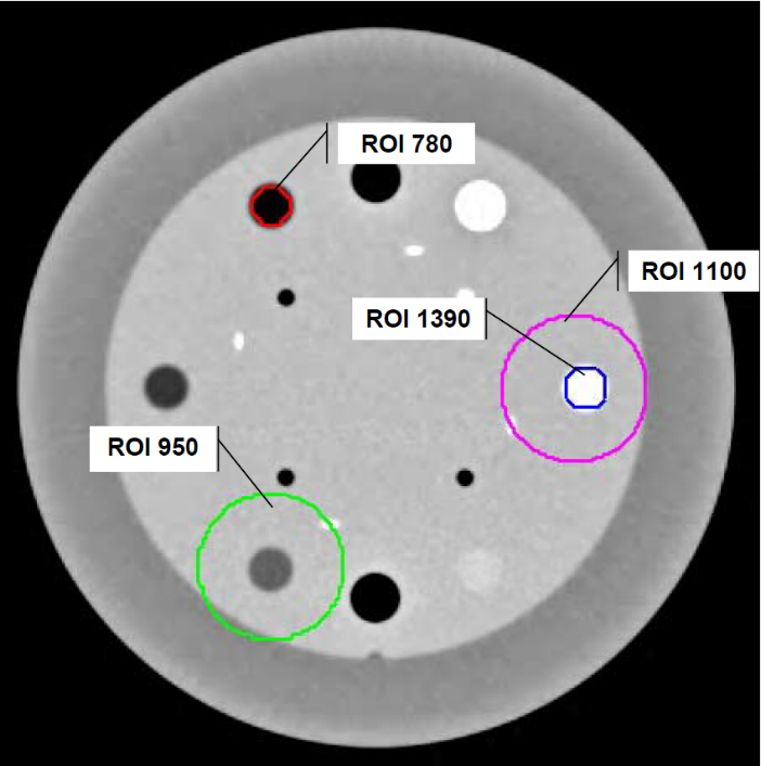
Figure 1: Axial slice from the phantom used in this investigation. The imaging protocol used for the CT data acquisition was our clinically used brain protocol, where the reconstructed voxel size is 0.976×0.976×1 mm3. The four ROIs used in this work for testing of the imaging feature variability dependence on the GLCM discretization are outlined on the figure. The nominal Hus for each ROI are also shown. Please note that ROI 1100 contains ROI 1390. While the ROI 1390 is fairly homogenous (~1.5% standard deviation of the HUs), the ROI 1100 is more variable (~6% standard deviation of the HUs). ROI 1390 has average HU of 1390, while the incorporation of other materials in the ROI 1100 brings the average HU for that ROI down to 1100
For each ROI four gray-level co-occurrence matrices (GLCMs) were created with an in-house software.31 Two of the GLCMs were with fixed number of bins, 32 and 64 respectively, while the other two used fixed bin width of 1 HU and 4 HU. In all for representations the GLCMs covered the entire range of HU characteristic for the ROI. The fixed bin number GLCMs had fixed size, while the fixed bin width GLCMs had variable sizes, depending on the ROI HU range. Eighteen commonly used image features were calculated from the four GLCMs. Those features included maximum, mean, variance, entropy, energy, IMC1, IMC2, auto correlation, cluster prominence, shade, contrast, correlation, tendency, dissimilarity, homogeneity 1, homogeneity 2, inverse difference moment normalized, and inverse difference normalized [8]. For each of those features its variability over the seven scans was estimated. The feature variability was defined as standard deviation of the feature normalized to the average of the feature. For presentation purposes the variabilities were converted into per-cent values.
III Feature comparisons and normalization
The feature variability was compared on ROI basis. Namely, for each ROI the feature variabilities were presented on a common plot. This representation allowed the separation of ROIs with more variable density against the ROIs with more uniform density. Furthermore, the variability of the GLCMs with higher resolutions were normalized to their counterparts with lower resolutions. Thereby, the variabilities of 1 HU and 4 HU GLCMs were compared, as well as the variabilities of 64 and 32 bin GLCMs on ROI-by-ROI basis. By performing this normalization, it was evaluated to what extent the noise, resulting from the fine resolution, affects the feature stability, depending on the GLCM discretization approach.
In addition, all the features were normalized on measurement-by-measurement (i.e. scan-by-scan) basis, and the variabilities of the normalized features were compared to the variabilities of the original (non-normalized) features. The tested normalizations included multiplication and division to the ROI volumes, as well as multiplication and division by the ROI ranges. The rationale behind the volume normalizations was that the investigated textural features are derived from GLCMs, which in turn are generated form volumetric objects differing in size. Therefore, the differences in size might affect the contents of the GLCMs, which in turn might affect the imaging features and in particular their variabilities. The range normalization hypothesis is rooted in the fact that all of the features are based on summations, which scale with the number of gray-levels in the GLCMs. Thereby, differences in the ranges from measurement-to-measurement would affect the GLCMs and the corresponding feature variability.
Results
I Feature variability dependence on GLCM discretization
The interplay between feature variability dependence and GLCM discretization approach is summarized on (figure 2) Close inspection of the figure indicates a noticeable contrast between the relations between the ROI homogeneity and the GLCM binning technique. The top two panels of the figure present the variabilities for the homogenous regions 780 and 1390 for all four GLCM representations, which are color coded in the figure legend. Notably, with all of the GLCM discretization’s the variabilities of the inverse difference moment normalized, and the inverse difference normalized are of the order of 0.5%. Because of the scale of the plot they are unnoticeable. As for the variabilities of the other features in majority of the cases the variability resulting from the fixed bin width GLCMs is larger than the variability of the fixed number of bins GLCMs. The picture is completely reversed for the variabilities in the more heterogeneous ROIs (ROIs 950 and 1100), plotted in the bottom two panels. In that case the variability of the fixed bin width GLCMs is substantially smaller than the variability exhibited by fixed number of bins GLCMs. Another interesting observation which can be made from the bottom two panels is that with increasing ROI heterogeneity the difference in variability between fixed number of bins and fixed bin width GLCMs increases. The variability of the HUs of ROI 950 (standard deviation of HUs normalized to nominal HU) is 4.2%, while the HU variability of ROI 1100 is 6.6%.
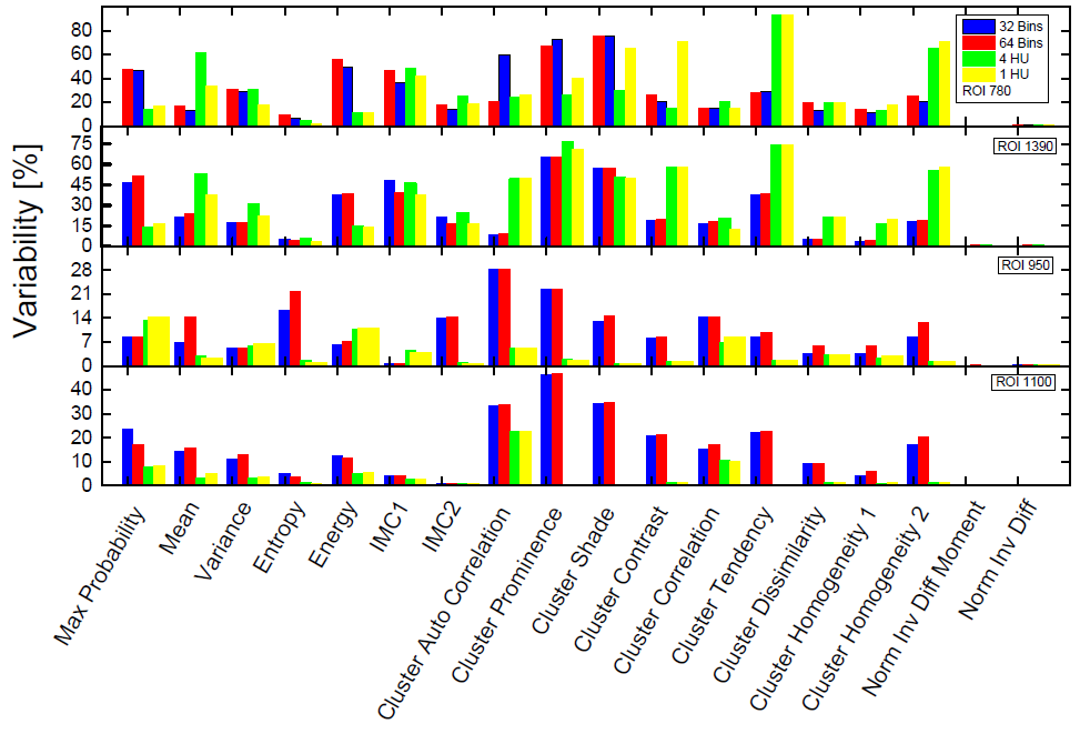
Figure 2: A composite bar plot of the variability of all 18 features for all ROIs, derived from all GLCM discretization representations. The type of the GLCM discretization is color coded in the figure legend, where also the ROI nominal HU is specified. The top two panels are for the more homogenous ROIs 780 and 1390, while the bottom two panels present the data for the more heterogeneous ROIs. The variability is expressed in percent. Note that for normalized inverse difference moment and the normalized inverse difference the variabilities are around and less than 1%, and thereby they too small for the scale of the plot.
II Feature variability dependence on GLCM bin width
Another aspect examined in this work is the GLCM variability dependence on the discretization resolution, since this resolution can affect the image noise (figure 3) presents the normalized variabilities for all four ROIs [21, 22, 39, 45]. The variability of the features derived from the 64 bin GLCMs have been normalized to the feature variability derived from 32 bin GLCMs (blue bars), while the variability of 1 HU GLCMs was normalized to the variability of the 4 HU GLCMs (red bars). In addition to the normalized variabilities in each panel of the figure the value of one is plotted as a dashed line to help the comparison. Fixed number of bins GLCMs demonstrate that with decreasing number of bins (from 64 to 32) and presumably decreasing nose the average (over all 18 features) normalized variability is 0.99, 0.98, 1.19, and 1.03 for ROIs 780, 1390, 950, and 1100. The average normalized variabilities between 1 HU and 4 HU GLCMs are 1.23, 0.92, 1.0, and 1.02 respectively. Those average normalized variabilities as well as the feature-by-feature data on Figure 3 indicate that the discretization bin size in the GLCM generation has rather minimal effect. There are only 4 out of 144 normalized feature variabilities where the difference from two to about four-fold.

Figure 3: Similarly, to Figure 2 this a composite bar plot, but this time for the normalized variabilities derived from the different GLCMs. The normalization is specified by color coding in the figure legend. The variability ratios are presented for each ROI separately in the corresponding figure panels. In addition to the dimensionless variability ration the value of one is also plotted in each panel with a dashed line. This indicates what is the relative ration of feature variability as a function of the GLCM discretization approach.
III Normalization effects on GLCM feature stability
The normalization dependence of the feature variability was examined for each ROI separately for all four GLCM representations. (Table 1) presents the variability dependence on normalization for ROI 780. Of the eighteen features studied only twelve exhibited variability dependences on the normalization. Those features are listed in the first column of the table. The next four columns outline what type of normalization reduces the feature variability for each GLCM representation – fixed bin widths of 1 HU and 4 HU, as well as fixed number of 64 and 32 bins respectively. The notations “*Volume” and “/Volume” indicate that the feature variability is reduced by multiplication or division by ROI volume respectively. Similarly, “*Range” and “/Range” reduce variability by multiplying or dividing by the ROI range. In the next set of four columns in the table the unnormalized variabilities of the imaging features are shown for each GLCM generation approach. Finally, in the last four columns the feature variability after the normalization is presented. The empty cells in the table indicate that for that particular GLCM no reduction of feature variability was observed after all normalization types were applied. The comparison of the unnormalized and normalized variabilities on feature-by-feature basis for each GLCM demonstrates the achievable reduction in variability after normalization. For example, the mean, the variance, the energy, and the auto correlation are weekly dependent on volume multiplication since the changes in their variabilities are small for all GLCM representations for ROI 780. The same is true for majority of the other features, but there are exceptions. For instance, cluster tendency and homogeneity 2 for fixed bin width GLCMs are very strongly affected by range, where normalization reduces variability almost in half.
Table 1: Normalization effects on the image feature variability for twelve features, derived from all GLCMs. The table is for the uniform density ROI 780. Only twelve of the eighteen investigated textural features are presented in the table since image feature variability was reduced only for those features. The first column outlines the feature type, the next four columns present the normalization type which reduces the feature variability, the subsequent four columns show the non-normalized feature variability (in percent), and the last four columns present the feature variability reduction after normalization. The normalization is “*Volume”, “/Volume”, “*Range”, and “/Range” where it is multiplication and division by ROI volume, as well as multiplication and division by ROI range respectively. The type of GLCM discretization is outlined in the second raw of the table.
|
|
Normalization type ROI 780 |
Variability ROI 780 [%] |
Variability ROI 780 normalized [%] |
|||||||||
|
|
1 HU |
4 HU |
64 Bins |
32 Bins |
1HU |
4 HU |
64 Bins |
32 Bins |
1 HU |
4 HU |
64 Bins |
32 Bins |
|
Mean |
*Volume |
*Volume |
*Volume |
*Volume |
33.13 |
61.34 |
13.62 |
16.89 |
31.55 |
59.66 |
11.90 |
15.62 |
|
Variance |
*Volume |
*Volume |
*Volume |
*Volume |
18.17 |
31.18 |
29.05 |
30.51 |
16.78 |
29.83 |
28.09 |
29.50 |
|
Energy |
*Volume |
*Volume |
*Volume |
*Volume |
11.04 |
10.96 |
48.90 |
55.89 |
9.81 |
9.70 |
47.64 |
54.46 |
|
Auto correlation |
*Volume |
*Volume |
*Volume |
*Volume |
26.47 |
24.60 |
59.96 |
20.39 |
25.06 |
23.19 |
58.31 |
20.32 |
|
Prominence |
/Range |
/Range |
/Range |
/Range |
40.19 |
26.24 |
72.11 |
66.74 |
38.13 |
17.82 |
56.24 |
48.19 |
|
Shade |
/Range |
/Range |
/Range |
/Range |
65.25 |
29.46 |
75.57 |
75.08 |
65.16 |
24.96 |
64.78 |
63.91 |
|
Contrast |
/Range |
/Range |
/Range |
/Range |
70.69 |
15.20 |
20.68 |
26.17 |
35.28 |
14.42 |
19.34 |
26.04 |
|
Correlation |
/Volume |
/Volume |
/Volume |
/Volume |
15.06 |
20.42 |
14.96 |
15.55 |
13.30 |
19.44 |
14.05 |
14.43 |
|
Tendency |
/Range |
/Range |
/Range |
/Range |
92.91 |
92.54 |
28.80 |
28.16 |
53.91 |
53.48 |
28.18 |
28.04 |
|
Dissimilarity |
/Range |
/Range |
|
|
19.39 |
19.38 |
12.97 |
19.29 |
19.09 |
19.17 |
|
|
|
Homogeneity 1 |
/Range |
/Range |
|
|
17.49 |
13.50 |
11.03 |
14.41 |
17.43 |
12.99 |
|
|
|
Homogeneity 2 |
/Range |
/Range |
/Range |
/Range |
70.37 |
65.32 |
20.39 |
24.89 |
34.96 |
30.20 |
19.06 |
24.74 |
Table 2 is similar to Table 1, but it presents the data for the other homogeneous region – ROI 1390. The feature variability is affected in similar fashion as for ROI 780, but this time the reduction in the variability of cluster tendency and homogeneity 2 is less pronounced than for the first homogeneous ROI. The common observation for the two ROIs is that all twelve features for almost all GLCM generation approaches are influenced by some type of normalization of the imaging feature.
The remaining tables (cf. Table 3 and Table 4) contain the data for the two heterogeneous regions – ROI 950 and ROI 1100. For fixed bin width GLCMs the mean the variance, and the energy demonstrate weak dependence of variability on volume. In the case of fixed bin width GLCMs for these features the variability is minimized by normalizing to the range as opposed to multiplication by volume as is was in the case with the homogeneous ROIs above. Furthermore, the variability of all other imaging (from auto correlation to homogeneity 2) features for the fixed number of bins GLCMs in table 3 and table 4 is consistently reduced when the features are multiplied by the range of the ROI, which is contrast with the behavior of the variability of those features in the former two tables, where normalization to range and volume, as well as no normalization reduce variability. The only other two features for which the variability is reduced by normalization in the case of fixed bin width GLCMs are the auto correlation and the correlation, where normalization to volume and multiplication to range respectively.
Table 2: The same as Table 1, but for the second uniform density ROI (ROI 1390).
|
|
Normalization type ROI 1390 |
Variability ROI 1390 [%] |
Variability ROI 1390 normalized [%] |
|||||||||
|
|
1 HU |
4 HU |
64 Bins |
32 Bins |
1HU |
4 HU |
64 Bins |
32 Bins |
1 HU |
4 HU |
64 Bins |
32 Bins |
|
Mean |
*Volume |
*Volume |
*Volume |
*Volume |
37.79 |
52.87 |
23.29 |
21.21 |
33.86 |
48.61 |
20.22 |
18.10 |
|
Variance |
*Volume |
*Volume |
*Volume |
*Volume |
21.92 |
30.99 |
17.17 |
17.31 |
18.34 |
27.25 |
16.79 |
16.96 |
|
Energy |
*Volume |
*Volume |
*Volume |
*Volume |
14.21 |
14.53 |
38.37 |
37.46 |
10.73 |
11.14 |
38.16 |
37.12 |
|
Auto correlation |
*Volume |
*Volume |
*Volume |
*Volume |
49.64 |
49.10 |
8.52 |
8.48 |
49.47 |
48.94 |
7.08 |
6.98 |
|
Prominence |
/Range |
/Range |
/Range |
/Range |
70.80 |
76.28 |
64.91 |
64.99 |
53.54 |
85.26 |
47.45 |
47.74 |
|
Shade |
/Range |
/Range |
/Range |
/Range |
50.15 |
50.23 |
57.22 |
57.35 |
47.05 |
47.15 |
39.33 |
39.71 |
|
Contrast |
/Range |
/Range |
/Range |
/Range |
57.96 |
57.56 |
18.88 |
18.88 |
38.57 |
38.10 |
11.88 |
12.18 |
|
Correlation |
/Volume |
/Volume |
/Volume |
/Volume |
12.39 |
20.12 |
17.87 |
16.30 |
10.54 |
18.61 |
16.38 |
14.59 |
|
Tendency |
/Range |
/Range |
/Range |
/Range |
74.01 |
73.84 |
37.66 |
37.66 |
56.35 |
56.12 |
18.29 |
18.56 |
|
Dissimilarity |
/Range |
/Range |
|
|
21.09 |
21.14 |
4.88 |
5.21 |
4.88 |
4.88 |
|
|
|
Homogeneity 1 |
/Range |
/Range |
|
|
19.41 |
15.70 |
4.04 |
3.68 |
5.54 |
8.36 |
|
|
|
Homogeneity 2 |
/Range |
/Range |
/Range |
/Range |
57.82 |
55.45 |
18.59 |
17.79 |
38.41 |
35.65 |
11.93 |
12.37 |
Table 3: The same as Table 1, but for the first heterogeneous ROI (ROI 950).
|
|
Normalization type ROI 950 |
Variability ROI 950 [%] |
Variability ROI 950 normalized [%] |
|||||||||
|
|
1 HU |
4 HU |
64 Bins |
32 Bins |
1HU |
4 HU |
64 Bins |
32 Bins |
1 HU |
4 HU |
64 Bins |
32 Bins |
|
Mean |
*Volume |
*Volume |
/Range |
/Range |
2.20 |
3.06 |
8.30 |
8.32 |
1.81 |
1.90 |
5.56 |
7.56 |
|
Variance |
*Volume |
*Volume |
/Range |
/Range |
6.56 |
5.77 |
14.36 |
6.98 |
6.11 |
5.07 |
7.06 |
5.60 |
|
Energy |
*Volume |
*Volume |
/Range |
/Range |
11.03 |
10.73 |
21.86 |
16.27 |
10.59 |
10.30 |
14.13 |
15.87 |
|
Auto correlation |
/Volume |
/Volume |
*Range |
*Range |
5.22 |
5.18 |
14.27 |
13.85 |
4.57 |
4.53 |
7.79 |
7.38 |
|
Prominence |
|
|
*Range |
*Range |
1.77 |
1.80 |
28.16 |
28.11 |
|
|
21.34 |
21.29 |
|
Shade |
|
|
*Range |
*Range |
0.71 |
0.73 |
22.45 |
22.43 |
|
|
15.31 |
15.29 |
|
Contrast |
|
|
*Range |
*Range |
1.30 |
1.25 |
14.52 |
13.01 |
|
|
6.99 |
5.46 |
|
Correlation |
*Range |
*Range |
*Range |
*Range |
8.52 |
6.83 |
8.33 |
8.21 |
2.23 |
2.97 |
5.40 |
7.11 |
|
Tendency |
|
|
*Range |
*Range |
1.49 |
1.50 |
14.34 |
14.18 |
|
|
6.76 |
6.58 |
|
Dissimilarity |
|
|
*Range |
*Range |
3.13 |
3.13 |
9.89 |
8.41 |
|
|
3.05 |
3.82 |
|
Homogeneity 1 |
|
|
*Range |
*Range |
2.88 |
2.32 |
5.81 |
3.52 |
|
|
2.72 |
2.26 |
|
Homogeneity 2 |
|
|
*Range |
*Range |
1.30 |
1.21 |
12.72 |
8.53 |
|
|
5.11 |
1.32 |
Table 4: The same as Table 1, but for the second heterogeneous ROI (ROI 1100)
|
|
Normalization type ROI 1100 |
Variability ROI 1100 [%] |
Variability ROI 1100 normalized [%] |
|||||||||
|
|
1 HU |
4 HU |
64 Bins |
32 Bins |
1HU |
4 HU |
64 Bins |
32 Bins |
1 HU |
4 HU |
64 Bins |
32 Bins |
|
Mean |
*Volume |
*Volume |
/Range |
/Range |
5.02 |
3.25 |
15.52 |
14.55 |
4.07 |
3.87 |
6.56 |
8.53 |
|
Variance |
*Volume |
*Volume |
/Range |
/Range |
3.47 |
3.10 |
13.15 |
11.13 |
3.27 |
3.01 |
3.98 |
5.19 |
|
Energy |
*Volume |
*Volume |
/Range |
/Range |
5.31 |
5.16 |
11.69 |
12.65 |
5.01 |
4.95 |
4.96 |
11.29 |
|
Auto correlation |
/Volume |
/Volume |
*Range |
*Range |
22.56 |
22.56 |
33.65 |
33.12 |
21.04 |
21.03 |
25.84 |
25.45 |
|
Prominence |
|
|
*Range |
*Range |
0.62 |
0.60 |
46.72 |
46.48 |
|
|
34.45 |
34.21 |
|
Shade |
|
|
*Range |
*Range |
0.61 |
0.59 |
34.53 |
34.37 |
|
|
22.56 |
22.39 |
|
Contrast |
|
|
*Range |
*Range |
1.42 |
1.43 |
21.33 |
20.69 |
|
|
9.97 |
9.38 |
|
Correlation |
*Range |
*Range |
*Range |
*Range |
10.37 |
10.52 |
17.29 |
15.38 |
5.23 |
3.26 |
6.72 |
7.49 |
|
Tendency |
|
|
*Range |
*Range |
0.51 |
0.51 |
22.57 |
22.44 |
|
|
11.06 |
10.94 |
|
Dissimilarity |
|
|
*Range |
*Range |
1.28 |
1.32 |
9.26 |
9.07 |
|
|
1.86 |
2.60 |
|
Homogeneity 1 |
|
|
*Range |
*Range |
1.19 |
1.01 |
5.97 |
4.34 |
|
|
4.68 |
6.25 |
|
Homogeneity 2 |
|
|
*Range |
*Range |
1.42 |
1.41 |
20.18 |
16.96 |
|
|
8.87 |
5.81 |
D i s c u s s i o n
The findings here in indicate that the variability of the imaging features derived from GLCMs depends on different factors. The first factor is the primary endpoint of this investigation – the GLCM discretization approach. The second factor is the feature normalization, where different normalization factors based on HU range or the volume of the textural object tend to reduce the imaging feature variability. The last factor that affects the imaging feature variability in conjunction with the first two factors mentioned above is the homogeneity of the textural object.
Our results suggest that for homogeneous ROIs the variability of the fixed number of bins GLCMs features was somewhat lower than the variability of the features derived from fixed bin width GLCMs. The situation was exactly opposite for heterogeneous ROIs, where the features derived from fixed bin width GLCMs showed lower variability. The standard deviation of the HU over the homogeneous ROIs was around 1.5%, while for the heterogeneous ROIs it was over 4%. This suggests that probably around HU standard deviation of 2% to 3% there is a discrimination between feature variability interplay with the GLCM discretization approach and homogeneity of the textural object.
To put that in perspective for application to real patients the data for HU variation for forty randomly chosen lung, head-and-neck (HN), prostate, and pancreas patients was compiled (ten per anatomical site). For each of those cases the HU standard deviation as well as the average HU value for the GTV, as outlined by the attending physician, was tallied. The HU variabilities for the lung, the HN, the prostate, and the pancreas cases ranged from 8% to 48%, 3.8% to 12.6%, 1.8% to 17%, and 1.9% to 26% respectively. Notably in one prostate and one pancreas cases the HU variability was as low as ~2%. These data suggest that for typical patient cases the use of textural features derived from fixed bin width GLCMs may be more suitable. Besides the fact the imaging feature variability for the fixed bin width GLCMs is lower for heterogeneous objects, the variability for fewer features is affected by different normalization factors. The date presented above indicate that only in five out of eighteen features the variability is reduced when scaling with object’s range for cluster contrast or volume for mean, variance, energy, and cluster auto correlation is employed.
Conclusions
Imaging biomarkers are an exciting new paradigm in cancer diagnosis and management. Successful application of those biomarkers requires comprehensive understanding of their properties and the effects of the different computational approaches, used to derive them. Biomarkers variability and susceptibility to different factors is an active area of research in the quantitative imaging community. In this work the variability of CT textural imaging features, derived from GLCMs, was investigated on phantom data. Thereby any physiological changes which may affect the presented results were excluded. It was found in the study that variability of twelve out of eighteen commonly used features is affected by the discretization approach of the image processing, where the features from fixed bin width GLCMs are influenced to a smaller extent than their counterparts derived from fixed number of bins GLCMs. This finding is very similar to the findings of other investigators, which discovered similar effect on positron emission tomography patient data.39 Furthermore, our phantom studies indicated that the two different discretization approaches in the GLCMs creation are affected differently depending on the homogeneity of the textural object. The fixed number of bins GLCMs produce less variable features for homogenous objects and vice-versa. Finally, the effects of different normalization parameters on the imaging feature variability were investigated and it was demonstrated that for realistic patient scenarios the use of fixed bin width GLCMs may be advantageous.
Conflict of Interests
None
Article Info
Article Type
Research ArticlePublication history
Received: Fri 31, Aug 2018Accepted: Tue 18, Sep 2018
Published: Fri 28, Sep 2018
Copyright
© 2023 Ivaylo Mihaylov. This is an open-access article distributed under the terms of the Creative Commons Attribution License, which permits unrestricted use, distribution, and reproduction in any medium, provided the original author and source are credited. Hosting by Science Repository.DOI: 10.31487/j.RDI.2018.10.005
Author Info
Corresponding Author
Ivaylo MihaylovDepartment of Radiation Oncology, University of Miami, USA
Figures & Tables
Table 1: Normalization effects on the image feature variability for twelve features, derived from all GLCMs. The table is for the uniform density ROI 780. Only twelve of the eighteen investigated textural features are presented in the table since image feature variability was reduced only for those features. The first column outlines the feature type, the next four columns present the normalization type which reduces the feature variability, the subsequent four columns show the non-normalized feature variability (in percent), and the last four columns present the feature variability reduction after normalization. The normalization is “*Volume”, “/Volume”, “*Range”, and “/Range” where it is multiplication and division by ROI volume, as well as multiplication and division by ROI range respectively. The type of GLCM discretization is outlined in the second raw of the table.
|
|
Normalization type ROI 780 |
Variability ROI 780 [%] |
Variability ROI 780 normalized [%] |
|||||||||
|
|
1 HU |
4 HU |
64 Bins |
32 Bins |
1HU |
4 HU |
64 Bins |
32 Bins |
1 HU |
4 HU |
64 Bins |
32 Bins |
|
Mean |
*Volume |
*Volume |
*Volume |
*Volume |
33.13 |
61.34 |
13.62 |
16.89 |
31.55 |
59.66 |
11.90 |
15.62 |
|
Variance |
*Volume |
*Volume |
*Volume |
*Volume |
18.17 |
31.18 |
29.05 |
30.51 |
16.78 |
29.83 |
28.09 |
29.50 |
|
Energy |
*Volume |
*Volume |
*Volume |
*Volume |
11.04 |
10.96 |
48.90 |
55.89 |
9.81 |
9.70 |
47.64 |
54.46 |
|
Auto correlation |
*Volume |
*Volume |
*Volume |
*Volume |
26.47 |
24.60 |
59.96 |
20.39 |
25.06 |
23.19 |
58.31 |
20.32 |
|
Prominence |
/Range |
/Range |
/Range |
/Range |
40.19 |
26.24 |
72.11 |
66.74 |
38.13 |
17.82 |
56.24 |
48.19 |
|
Shade |
/Range |
/Range |
/Range |
/Range |
65.25 |
29.46 |
75.57 |
75.08 |
65.16 |
24.96 |
64.78 |
63.91 |
|
Contrast |
/Range |
/Range |
/Range |
/Range |
70.69 |
15.20 |
20.68 |
26.17 |
35.28 |
14.42 |
19.34 |
26.04 |
|
Correlation |
/Volume |
/Volume |
/Volume |
/Volume |
15.06 |
20.42 |
14.96 |
15.55 |
13.30 |
19.44 |
14.05 |
14.43 |
|
Tendency |
/Range |
/Range |
/Range |
/Range |
92.91 |
92.54 |
28.80 |
28.16 |
53.91 |
53.48 |
28.18 |
28.04 |
|
Dissimilarity |
/Range |
/Range |
|
|
19.39 |
19.38 |
12.97 |
19.29 |
19.09 |
19.17 |
|
|
|
Homogeneity 1 |
/Range |
/Range |
|
|
17.49 |
13.50 |
11.03 |
14.41 |
17.43 |
12.99 |
|
|
|
Homogeneity 2 |
/Range |
/Range |
/Range |
/Range |
70.37 |
65.32 |
20.39 |
24.89 |
34.96 |
30.20 |
19.06 |
24.74 |
Table 2: The same as Table 1, but for the second uniform density ROI (ROI 1390).
|
|
Normalization type ROI 1390 |
Variability ROI 1390 [%] |
Variability ROI 1390 normalized [%] |
|||||||||
|
|
1 HU |
4 HU |
64 Bins |
32 Bins |
1HU |
4 HU |
64 Bins |
32 Bins |
1 HU |
4 HU |
64 Bins |
32 Bins |
|
Mean |
*Volume |
*Volume |
*Volume |
*Volume |
37.79 |
52.87 |
23.29 |
21.21 |
33.86 |
48.61 |
20.22 |
18.10 |
|
Variance |
*Volume |
*Volume |
*Volume |
*Volume |
21.92 |
30.99 |
17.17 |
17.31 |
18.34 |
27.25 |
16.79 |
16.96 |
|
Energy |
*Volume |
*Volume |
*Volume |
*Volume |
14.21 |
14.53 |
38.37 |
37.46 |
10.73 |
11.14 |
38.16 |
37.12 |
|
Auto correlation |
*Volume |
*Volume |
*Volume |
*Volume |
49.64 |
49.10 |
8.52 |
8.48 |
49.47 |
48.94 |
7.08 |
6.98 |
|
Prominence |
/Range |
/Range |
/Range |
/Range |
70.80 |
76.28 |
64.91 |
64.99 |
53.54 |
85.26 |
47.45 |
47.74 |
|
Shade |
/Range |
/Range |
/Range |
/Range |
50.15 |
50.23 |
57.22 |
57.35 |
47.05 |
47.15 |
39.33 |
39.71 |
|
Contrast |
/Range |
/Range |
/Range |
/Range |
57.96 |
57.56 |
18.88 |
18.88 |
38.57 |
38.10 |
11.88 |
12.18 |
|
Correlation |
/Volume |
/Volume |
/Volume |
/Volume |
12.39 |
20.12 |
17.87 |
16.30 |
10.54 |
18.61 |
16.38 |
14.59 |
|
Tendency |
/Range |
/Range |
/Range |
/Range |
74.01 |
73.84 |
37.66 |
37.66 |
56.35 |
56.12 |
18.29 |
18.56 |
|
Dissimilarity |
/Range |
/Range |
|
|
21.09 |
21.14 |
4.88 |
5.21 |
4.88 |
4.88 |
|
|
|
Homogeneity 1 |
/Range |
/Range |
|
|
19.41 |
15.70 |
4.04 |
3.68 |
5.54 |
8.36 |
|
|
|
Homogeneity 2 |
/Range |
/Range |
/Range |
/Range |
57.82 |
55.45 |
18.59 |
17.79 |
38.41 |
35.65 |
11.93 |
12.37 |
Table 3: The same as Table 1, but for the first heterogeneous ROI (ROI 950).
|
|
Normalization type ROI 950 |
Variability ROI 950 [%] |
Variability ROI 950 normalized [%] |
|||||||||
|
|
1 HU |
4 HU |
64 Bins |
32 Bins |
1HU |
4 HU |
64 Bins |
32 Bins |
1 HU |
4 HU |
64 Bins |
32 Bins |
|
Mean |
*Volume |
*Volume |
/Range |
/Range |
2.20 |
3.06 |
8.30 |
8.32 |
1.81 |
1.90 |
5.56 |
7.56 |
|
Variance |
*Volume |
*Volume |
/Range |
/Range |
6.56 |
5.77 |
14.36 |
6.98 |
6.11 |
5.07 |
7.06 |
5.60 |
|
Energy |
*Volume |
*Volume |
/Range |
/Range |
11.03 |
10.73 |
21.86 |
16.27 |
10.59 |
10.30 |
14.13 |
15.87 |
|
Auto correlation |
/Volume |
/Volume |
*Range |
*Range |
5.22 |
5.18 |
14.27 |
13.85 |
4.57 |
4.53 |
7.79 |
7.38 |
|
Prominence |
|
|
*Range |
*Range |
1.77 |
1.80 |
28.16 |
28.11 |
|
|
21.34 |
21.29 |
|
Shade |
|
|
*Range |
*Range |
0.71 |
0.73 |
22.45 |
22.43 |
|
|
15.31 |
15.29 |
|
Contrast |
|
|
*Range |
*Range |
1.30 |
1.25 |
14.52 |
13.01 |
|
|
6.99 |
5.46 |
|
Correlation |
*Range |
*Range |
*Range |
*Range |
8.52 |
6.83 |
8.33 |
8.21 |
2.23 |
2.97 |
5.40 |
7.11 |
|
Tendency |
|
|
*Range |
*Range |
1.49 |
1.50 |
14.34 |
14.18 |
|
|
6.76 |
6.58 |
|
Dissimilarity |
|
|
*Range |
*Range |
3.13 |
3.13 |
9.89 |
8.41 |
|
|
3.05 |
3.82 |
|
Homogeneity 1 |
|
|
*Range |
*Range |
2.88 |
2.32 |
5.81 |
3.52 |
|
|
2.72 |
2.26 |
|
Homogeneity 2 |
|
|
*Range |
*Range |
1.30 |
1.21 |
12.72 |
8.53 |
|
|
5.11 |
1.32 |
Table 4: The same as Table 1, but for the second heterogeneous ROI (ROI 1100)
|
|
Normalization type ROI 1100 |
Variability ROI 1100 [%] |
Variability ROI 1100 normalized [%] |
|||||||||
|
|
1 HU |
4 HU |
64 Bins |
32 Bins |
1HU |
4 HU |
64 Bins |
32 Bins |
1 HU |
4 HU |
64 Bins |
32 Bins |
|
Mean |
*Volume |
*Volume |
/Range |
/Range |
5.02 |
3.25 |
15.52 |
14.55 |
4.07 |
3.87 |
6.56 |
8.53 |
|
Variance |
*Volume |
*Volume |
/Range |
/Range |
3.47 |
3.10 |
13.15 |
11.13 |
3.27 |
3.01 |
3.98 |
5.19 |
|
Energy |
*Volume |
*Volume |
/Range |
/Range |
5.31 |
5.16 |
11.69 |
12.65 |
5.01 |
4.95 |
4.96 |
11.29 |
|
Auto correlation |
/Volume |
/Volume |
*Range |
*Range |
22.56 |
22.56 |
33.65 |
33.12 |
21.04 |
21.03 |
25.84 |
25.45 |
|
Prominence |
|
|
*Range |
*Range |
0.62 |
0.60 |
46.72 |
46.48 |
|
|
34.45 |
34.21 |
|
Shade |
|
|
*Range |
*Range |
0.61 |
0.59 |
34.53 |
34.37 |
|
|
22.56 |
22.39 |
|
Contrast |
|
|
*Range |
*Range |
1.42 |
1.43 |
21.33 |
20.69 |
|
|
9.97 |
9.38 |
|
Correlation |
*Range |
*Range |
*Range |
*Range |
10.37 |
10.52 |
17.29 |
15.38 |
5.23 |
3.26 |
6.72 |
7.49 |
|
Tendency |
|
|
*Range |
*Range |
0.51 |
0.51 |
22.57 |
22.44 |
|
|
11.06 |
10.94 |
|
Dissimilarity |
|
|
*Range |
*Range |
1.28 |
1.32 |
9.26 |
9.07 |
|
|
1.86 |
2.60 |
|
Homogeneity 1 |
|
|
*Range |
*Range |
1.19 |
1.01 |
5.97 |
4.34 |
|
|
4.68 |
6.25 |
|
Homogeneity 2 |
|
|
*Range |
*Range |
1.42 |
1.41 |
20.18 |
16.96 |
|
|
8.87 |
5.81 |
References
1. Aerts HJ, Velazquez ER, Leijenaar RT, Parmar C, Grossmann P, et al. (2014) Decoding tumour phenotype by noninvasive imaging using a quantitative radiomics approach. Nat Commun 5: 4006. [Crossref]
2. Gillies RJ, Anderson AR, Gatenby RA, Morse DL (2010) The biology underlying molecular imaging in oncology: from genome to anatome and back again. Clin Radiol 65: 517-521. [Crossref]
3. Lambin P, Rios-Velazquez E, Leijenaar R, Carvalho S, van Stiphout RG, et al. (2012) Radiomics: Extracting more information from medical images using advanced feature analysis. Eur J Cancer 48: 441-446. [Crossref]
4. Cunliffe A, Armato SG 3rd, Castillo R, Pham N, Guerrero T, et al. (2015) Lung texture in serial thoracic computed tomography scans: correlation of radiomics-based features with radiation therapy dose and radiation pneumonitis development. Int J Radiat Oncol Biol Phys 91: 1048-1056. [Crossref]
5. He X, Sahiner B, Gallas BD, Chen W, Petrick N (2014) Computerized characterization of lung nodule subtlety using thoracic CT images. Phys Med Biol 59: 897-910. [Crossref]
6. Raman SP, Chen Y, Schroeder JL, Huang P, Fishman EK (2014) texture analysis of renal masses: pilot study using random forest classification for prediction of pathology. Acad Radiol 21: 1587-1596. [Crossref]
7. Lambin P, van Stiphout RG, Starmans MH, Rios-Velazquez E, Nalbantov G et al. (2013) Predicting outcomes in radiation oncology--multifactorial decision support systems. Nat Rev Clin Oncol 10: 27-40. [Crossref]
8. Leijenaar RT, Carvalho S, Velazquez ER, van Elmpt WJ, Parmar C, et al. (2013) Stability of FDG-PET Radiomics features: an integrated analysis of test-retest and inter-observer variability. Acta Oncol 52: 1391-1397. [Crossref]
9. N Ahuja, A Rosenfeld (1978) Note on the Use of 2nd-Order Gray-Level Statistics for Threshold Selection. Ieee T Syst Man Cyb 8: 895-898.
10. Buckler AJ, Bresolin L, Dunnick NR, Sullivan DC, Group (2011) A collaborative enterprise for multi-stakeholder participation in the advancement of quantitative imaging. Radiology 258: 906-914. [Crossref]
11. Coroller TP, Grossmann P, Hou Y, Rios Velazquez E, Leijenaar RT, et al. (2015) CT-based radiomic signature predicts distant metastasis in lung adenocarcinoma. Radiother Oncol 114: 345-350. [Crossref]
12. I El Naqa, P Grigsby, A Apte, E Kidd, E Donnelly, et al. (2009) Exploring feature-based approaches in PET images for predicting cancer treatment outcomes. Pattern Recognit 42: 1162-1171. [Crossref]
13. Ganeshan B, Panayiotou E, Burnand K, Dizdarevic S, Miles K (2012) Tumour heterogeneity in non-small cell lung carcinoma assessed by CT texture analysis: a potential marker of survival. Eur Radiol 22: 796-802. [Crossref]
14. Kawata Y, Niki N, Ohmatsu H, Kusumoto M, Tsuchida T, et al. (2012) Quantitative classification based on CT histogram analysis of non-small cell lung cancer: correlation with histopathological characteristics and recurrence-free survival. Med phys 39: 988-1000. [Crossref]
15. Kumar V, Gu Y, Basu S, Berglund A, Eschrich SA, et al. (2012) Radiomics: the process and the challenges. Magn Reson Imaging 30: 1234-1248. [Crossref]
16. Lambin P, Rios-Velazquez E, Leijenaar R, Carvalho S, van Stiphout RG, et al. (2012) Radiomics: extracting more information from medical images using advanced feature analysis. Eur J Cancer 48: 441-446. [Crossref]
17. Rafat M, Ali R, Graves EE (2015) Imaging radiation response in tumor and normal tissue. Am J Nucl Med Mol Imaging 5: 317-332. [Crossref]
18. Rose CJ1, Mills SJ, O'Connor JP, Buonaccorsi GA, Roberts C, et al. (2009) Quantifying spatial heterogeneity in dynamic contrast-enhanced MRI parameter maps. Magn Reson Med 62: 488-499. [Crossref]
19. Schacht DV, Drukker K, Pak I, Abe H, Giger ML (2015) Using quantitative image analysis to classify axillary lymph nodes on breast MRI: A new application for the Z 0011 Era. Eur J Radiol 84: 392-397. [Crossref]
20. Sun W, Tseng TL, Qian W, Zhang J, Saltzstein EC, et al. (2015) Using multiscale texture and density features for near-term breast cancer risk analysis. Med phys 42: 2853-2862. [Crossref]
21. Tixier F, Hatt M, Le Rest CC, Le Pogam A, Corcos L, et al. (2012) Reproducibility of tumor uptake heterogeneity characterization through textural feature analysis in 18F-FDG PET. J Nucl Med 53: 693-700. [Crossref]
22. Tixier F1, Le Rest CC, Hatt M, Albarghach N, Pradier O, et al. (2011) Intratumor heterogeneity characterized by textural features on baseline 18F-FDG PET images predicts response to concomitant radiochemotherapy in esophageal cancer. J Nucl Med 52: 369-378. [Crossref]
23. Qing-Gang Xu, Jun-Fang Xian (2015) Role of Quantitative Magnetic Resonance Imaging Parameters in the Evaluation of Treatment Response in Malignant Tumors. Chin Med J 128: 1128-1133. [Crossref]
24. Dehing-Oberije C, Aerts H, Yu S, De Ruysscher D, Menheere P, et al. (2011) Development and Validation of a Prognostic Model Using Blood Biomarker Information for Prediction of Survival of Non Small-Cell Lung Cancer Patients Treated with Combined Chemotherapy and Radiation or Radiotherapy Alone (Nct00181519, Nct00573040, and Nct00572325). Int J Radiat Oncol Biol Phys 81: 360-368. [Crossref]
25. Eisenhauer EA1, Therasse P, Bogaerts J, Schwartz LH, Sargent D, et al. (2009) New response evaluation criteria in solid tumours: revised RECIST guideline (version 1.1). Eur J Cancer 45: 228-247. [Crossref]
26. Therasse P, Arbuck SG, Eisenhauer EA, Wanders J, Kaplan RS, et al. (2000) New guidelines to evaluate the response to treatment in solid tumors. European Organization for Research and Treatment of Cancer, National Cancer Institute of the United States, National Cancer Institute of Canada. J Natl Cancer Inst 92: 205-216. [Crossref]
27. Hunter LA, Krafft S, Stingo F, Choi H, Martel MK, et al. (2013) High quality machine-robust image features: identification in nonsmall cell lung cancer computed tomography images. Medi phys 40: 121916. [Crossref]
28. Davnall F, Yip CS, Ljungqvist G, Selmi M, Ng F, et al. (2012) Assessment of tumor heterogeneity: an emerging imaging tool for clinical practice? Insights Imaging 3: 573-589. [Crossref]
29. DA Clausi (2002) An analysis of co-occurrence texture statistics as a function of grey level quantization. Can J Remote Sens 28: 45-62.
30. M. M. Gallowey (1975) Texture analysis using gray level run lengths. Computer Graphics and Image Processing 4: 172-179.
31. RM Haralick, Shanmuga K, I Dinstein (1973) Textural Features for Image Classification. Ieee T Syst Man Cyb Smc 3: 610-621.
32. L. K. Soh, C. Tsatsoulis (1999) Texture analysis of SAR sea ice imagery using gray level co-occurrence matrices Ieee T Geosci Remote 37: 780-795.
33. Galavis PE, Hollensen C, Jallow N, Paliwal B, Jeraj R (2010) Variability of textural features in FDG PET images due to different acquisition modes and reconstruction parameters. Acta Oncologica 49: 1012-1016. [Crossref]
34. Ganeshan B, Miles KA (2013) Quantifying tumour heterogeneity with CT. Cancer imaging 13: 140-149. [Crossref]
35. Zhao B, Tan Y, Tsai WY, Qi J, Xie C, et al. (2016) Reproducibility of radiomics for deciphering tumor phenotype with imaging. Sci Rep 6: 23428. [Crossref]
36. S Basu, LO Hall, DB Goldgof, YH Gu, V Kumar, et al. (2011) Developing a Classifier Model for Lung Tumors in CT-scan Images. Ieee Sys Man Cybern: 1306-1312.
37. Mackin D, Fave X, Zhang L, Fried D, Yang J, et al. (2015) Measuring Computed Tomography Scanner Variability of Radiomics Features. Invest Radiol 50: 757-765. [Crossref]
38. Zhao B, Tan Y, Tsai WY, Schwartz LH, Lu L (2014) Exploring Variability in CT Characterization of Tumors: A Preliminary Phantom Study. Transl Oncol 7: 88-93. [Crossref]
39. Leijenaar RT, Nalbantov G, Carvalho S, van Elmpt WJ, Troost EG, et al. (2015) The effect of SUV discretization in quantitative FDG-PET Radiomics: the need for standardized methodology in tumor texture analysis. Sci Rep 5: 11075. [Crossref]
40. Cook GJ, Yip C, Siddique M, Goh V, Chicklore S, et al. (2013) Are Pretreatment F-18-FDG PET Tumor Textural Features in Non-Small Cell Lung Cancer Associated with Response and Survival After Chemoradiotherapy? J Nucl Med 54: 19-26. [Crossref]
41. Dong X, Xing L, Wu P, Fu Z, Wan H, et al. (2013) Three-dimensional positron emission tomography image texture analysis of esophageal squamous cell carcinoma: relationship between tumor F-18-fluorodeoxyglucose uptake heterogeneity, maximum standardized uptake value, and tumor stage. Nucl Med Commun 34: 40-46. [Crossref]
42 Vaidya M, Creach KM, Frye J, Dehdashti F, Bradley JD, et al. (2012) Combined PET/CT image characteristics for radiotherapy tumor response in lung cancer. Radiother Oncol 102: 239-245. [Crossref]
43. Yang F, Thomas MA, Dehdashti F, Grigsby PW (2013) Temporal analysis of intratumoral metabolic heterogeneity characterized by textural features in cervical cancer. Eur J Nucl Med Mol Imaging 40: 716-727. [Crossref]
44. Oliver JA, Budzevich M, Zhang GG, Dilling TJ, Latifi K, et al. (2015) Variability of Image Features Computed from Conventional and Respiratory-Gated PET/CT Images of Lung Cancer. Transl Oncol 8: 524-534. [Crossref]
45. Huynh E, Coroller TP, Narayan V, Agrawal V, Hou Y, et al. (2016) CT-based radiomic analysis of stereotactic body radiation therapy patients with lung cancer. Radiother Oncol 120: 258-266. [Crossref]