CPU-GPU Rendering of CT Scan Images for Vertebra Reconstruction from CT Scan Images with a Calibration Policy
A B S T R A C T
In this work GPU implementation of classic 3D visualization algorithms namely Marching Cubes and Raycasting has been carried for cervical vertebra using VTK libraries. A proposed framework has been introduced for efficient and duly calibrated 3D reconstruction using Dicom Affine transform and Python Mayavi framework to address the limitation of benchmark visualization techniques i.e. lack of calibration, surface reconstruction artifacts and latency.
Keywords
Tomographic Imaging, 3D Reconstruction, MRI, CT Scan
Introduction
During the past decade immense work has been carried out in maturing tomographic imaging. Benchmark 3D visualization algorithms have been offloaded to GPUs in order to reduce latency and improving performance. In this field, frameworks like VTK has played a pivotal role and has emerged as a sole framework providing one stop solution to medical imaging. 3D slicer is another free to use software package available for medical image visualization. However, there still exists a room for improvement in producing accurately constructed 3D models and decreasing latency for 3D point cloud mesh generation. 3D medical imaging is evolving as a necessary tool for doctors to draw conclusive inference about an ailment. Today most commonly used platforms for medical imaging and analysis include CT Scan and MRI. CT scans are X Ray images which capture 360-degree view of human body and are approximately 5 mm apart. However, type of scan is a property of different CT scan machine manufacturers. MRI on the other hand is a completely harmless technique which uses magnetic fields to realign protons of different tissues. These protons when return to their original state at varying rate produce radio waves which are collected by the detectors. Therefore, all the tissues are captured in a layered manner using MRI imaging [1].
3D visualization and 3D reconstruction are two different aspects. In visualization there is no need for the reconstructed model to be accurate with regards to reconstruction. However, 3D reconstruction may require models accuracy. For 3D visualization specially in tomographic imaging, benchmark algorithms have been developed over a period of time ranging from simplest techniques like Surface Shaded Display (SSD), CPR, MIP to more elaborate algorithms like Raycasting, Raytracing and Marching cubes. Raycasting and marching cubes algos were much deliberated upon in 1990s, however, due to non-availability of matching computational power, implementation of these algorithms in tomography have surfaced to the desirable level until recently.
Literature Review
Famous 3D rendering and visualization techniques in tomographic imaging are Ray tracing, ray casting, surface shaded display and marching cubes [1]. Ray tracing is a surface rendering algorithm in which it is assumed that a ray is cast from the viewer to the object of interest. All the points on the object that are hit by the ray are sorted and the closest point is selected as the surface point. The surface point is then shaded using phong shading algorithm. Improvements to Raycasting algorithms have remained a topic of discussion during 1990s. In this era an improved model for the algorithm was finally presented by which addresses the three issues in the algorithm including shadows definition, modeling reflection and refractions [2]. Simply stated in ray casting a ray is assumed to be cast on a sphere and the points where the ray intersects the sphere are noted. Amongst these points the nearest point is registered which is less distant than the other point a diameter away. Similarly, surface shaded display produces depth perception by shading the surface in a way that surfaces nearer to the screen appear brighter. In SSD the surface is segmented as foreground and background. Surface gradients and normals are calculated which are then compared with the threshold to extract the desired surface. For shading purposes, phong shading is utilized.
Raycasting sometimes also known as raytracing is a popular algorithm developed in 1980s - 90s. Owing to the huge computation requirement parallel computation approaches for the algorithm have been sought over the time initially using pipelined approaches and then using GPUs. The main difference between ray casting and ray tracing is that ray casting is a volume rendering algorithm while ray tracing is surface rendering within built iteration. In raycasting the closest point is not selected, rather the ray bisects the volume and at evenly located points the color and opacity are interpolated. These interpolated values are then merged to produce the color at the pixel on the image plane. The algorithm presented by Blinn and Kajiya in their papers and derives an equation for intensity of light [3, 4]. For computer graphics a popular practical implementation for raycasting algorithm has been provided by Marc Levoy [5]. In his work Marc Levoy has introduced adaptive solution for calculating opacity and shading of voxels using a pipelined approach. Both opacity and shading are then merged to provide realistic 3D tomography. In order to acquire surface shading surface gradient is used to obtain surface normal which is fed in Phong’s shading model to get intensities.
Since completely homogeneous regions provide unreliable shading therefore opacity values obtained for such regions are multiplied with the surface gradient. The product obtained is zero for completely homogeneous regions which makes such regions transparent thus avoiding ill effects of inconsistency due to such regions. Opacity of voxels is obtained using simple formula analogous to central difference of current and neighboring voxels. Triangulation of intensity values from neighboring pixels produce opacity for the voxel under consideration. Complexity in 3D reconstruction by using mathematical modeling approaches has been reduced by using texture tracing technique [6]. The method has been explained in by first analysing 2D reconstruction using rectangles and then extrapolating the technique to 3D reconstruction using cubes [7].
A 3D object is assumed to be made of cubes [6]. If the 3D space in which the object of interest lies is considered to be made of a number of cubes of which the object is also a part but with different color only, then it can be easily perceived that there will be three types of cubes. The first type will be ones which lie within the surface completely. The second type of cubes will be the ones that lie completely outside the object whereas the third type will be those cubes which make part of both the object and the surrounding space. Third type of cubes will be intersected by the object surface. These three types of cubes have 8 vertices each which either lie inside the surface or are outliers. Therefore, the vertices have two states at a time. The surface intersects the cube in 28, 256 ways which are reduced to 14 cases keeping in view topology, rotation and reflection of thus formed triangles. These 14 cases are indexed using a binary code represented by 8 vertices, thus forming a look up table. Pattern of the binary code indicates one of the 14 cases for surface construction. Once the surface-cube interaction is known then comes the question of shading the surface. Unit normals to the triangulated surface are used for Gouraud shading.
I Marching Cubes Rendering on GPU Using VTK
For comparison of the two benchmark techniques CT scan dataset was obtained from Bone and Joint CT Scan Dataset [8]. Initially the obtained Dataset was converted into Housenfield Units and soft tissues were filtered out as in (Figure 1). The CT Scan Images as visualized in 3D with slices laid on the top of each other can be viewed in (Figure 2). Marching cubes (MC) algorithm sweeps a cube across these slices to reconstruct the 3d model. MC algorithm is an algorithmic manifestation of the famous quote of Michelangelo I saw the angel in the marble and carved until I set him free. The main idea is to move a cube across the slice slab. Point intersecting with the cube are converted to triangular surfaces shaded using shading algorithm. Slice slab as shown in (Figure 2) was used as an input to Python Sklearn package. CPU based reconstruction of Cervical c-2 vertebra commonly known as axis in shown in (Figure 3).
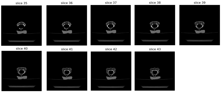
Figure 1: CT Scan Slices.
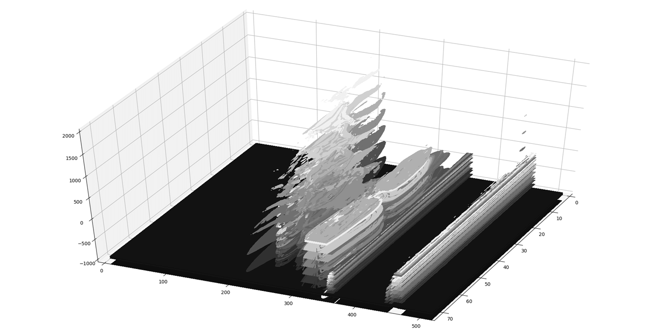
Figure 2: Overlaying CT slices.
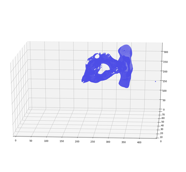
Figure 3: Marching Cubes CPU Implementation.
Python VTK 8.0 framework provides an accelerator for Marching cubes algorithm as shown in (Figure 4). Skimage package of Python provides a CPU implementation of the same algorithm. Both packages were used for simulations of Cervical C-2 vertebra. VTK based GPU rendered model surpasses CPU implementation both in terms of clarity and latency. Marching Cubes implementation on GPU takes approx 2 seconds for the first simulation.
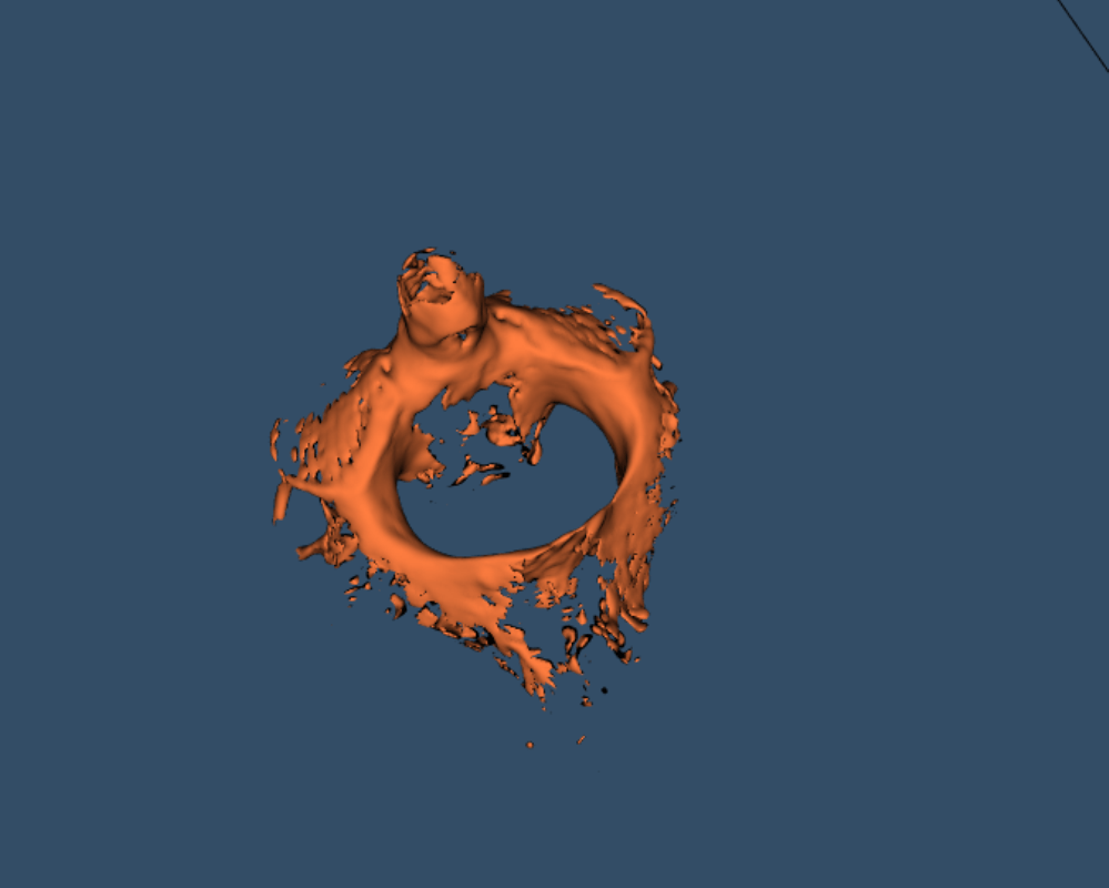
Figure 4: Cervical c-2 GPU Rendering Marching Cubes.
II RayCasting Implementation on GPU Using VTK
Raycasting is a volumetric reconstruction technique as opposed to the marching cube which is a surface reconstruction algorithm. Python sklearn library used for cervical reconstruction using raycasting took almost 5 minutes on Intel Core i5 processor (QuadCore). Immense latency reduction was observed while using NVIDIA GEFORCE GTX 1050 GPU (Figure 5). It was observed that as opposed to 300 seconds for CPU implementation, GPU implementation took approx 10 seconds for the first simulation whereas only 2 seconds for subsequent simulations.
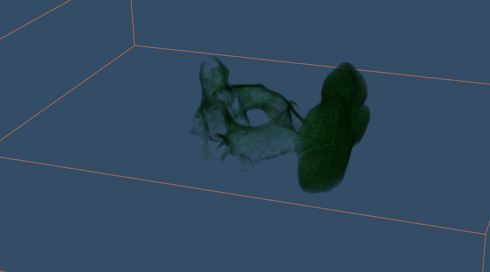
Figure 5: Cervical c-2 GPU Rendering RayCast.
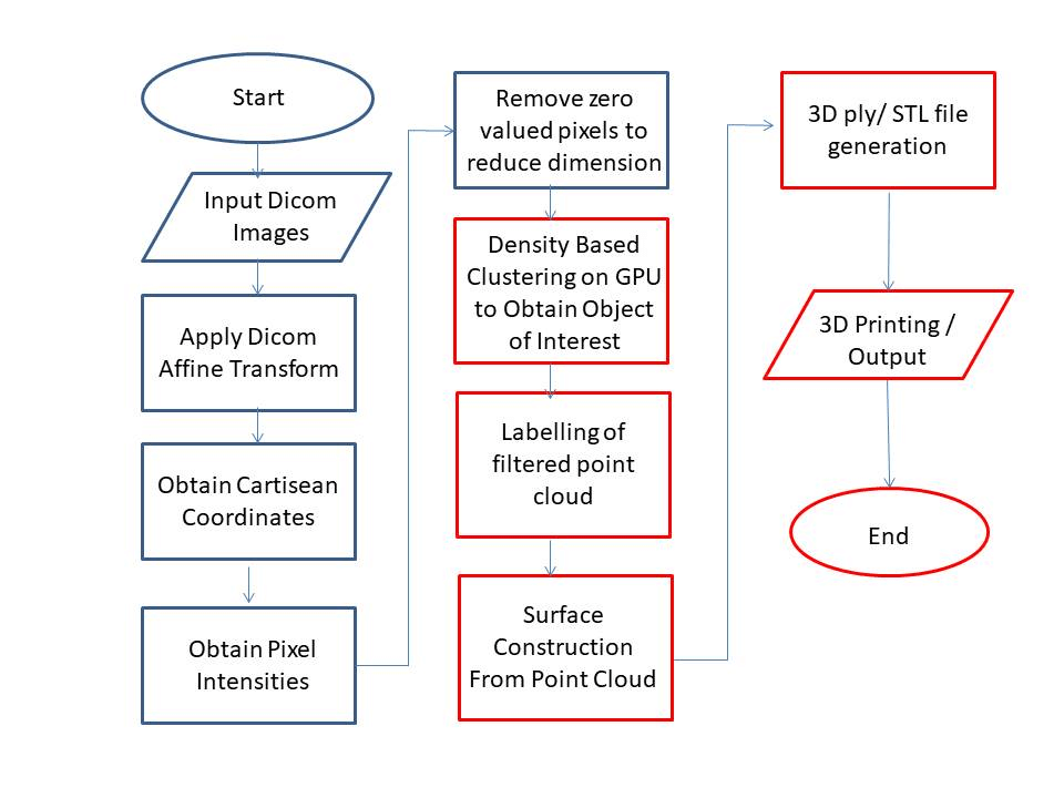
Figure 6: Proposed Algorithm for CT Scan Point Cloud Reconstruction.
In the field of medical 3D imaging, the main focus of both point cloud and surface reconstruction has remained on voxel interpolations. However, a powerful framework is available for camera images 3D reconstruction. Dicom format provides the needed tags required for mapping of a 2D dicom image point to 3D Reference Coordinate System. These dicom tags are read and converted to the Dicom Affine Matrix which is the transformation matrix used to transform 2D image points to 3D RCS Coordinates.
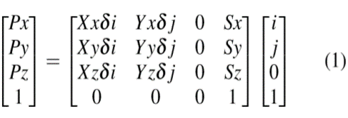
Parameters in this matrix multiplication are:
i. Xx, Xy, Xz are the Image Orientation values denote by dicom tag (0020,0037).
ii. δi and δ j are the column and row pixel spacing denoted by tags (0028,0030).
iii. Sx; Sy; Sz are the three values of image position denoted by tag (0020, 0032) and is located in mm from origin.
In order to read these tags Pydicom package has been used and algorithm of (Figure 6) followed. Listing of the code to obtain pixel data, image position and image orientation tags is given below:
$$ image = pydicom . dcmread ( dirName+”nn”+ filename , force = True ) image . file meta$$
$$ TransferSyntaxUID = pydicom.uid.ImplicitVRLittleEndian pixel data.append$$
$$( image . p i x e l a r r ay) image position.append ( image.ImagePositionPatient)$$
$$ imageorientation.append(image.ImageOrientationPatient) $$
To calculate the matrix in equation 1, we used numpy dot multiplication.
$$ o r i e n t a t i o n o f s l i c e = np . array ( image orientation ) $$
$$ Xxyz = o r i e n t a t i o n o f s l i c e [ 0 ] [ 0 : 3 ]$$
$$ Yxyz = o r i e n t a t i o n o f s l i c e [ 0 ] [ 3 : 6 ] $$
$$ Sxyz = np . array ( image position ) pixel spacing = image . PixelSpacing $$
$$ DeltaX = pixel spacing [0] DeltaY = pixel spacing [1]$$
However, the idea is to get the 3D coordinates of a pixel whose 2D coordinates are available in dicom image. So in actual we need to map stack of P 2D images of NxM size to NxMxPx4 matrix. Where, no. 4 represents the size of Dicom Affine Matrix. Reference database (8). The final matrix thus is of size NxMxPx4 where N = M = 512; P = 95. After applying affine transform to the input dicom images, the x,y,z coordinates and the voxel intensities at their respective coordinates were obtained. Vertebra point clouds produced from affine transform using Python’s Mayavi GPU based graphic and rendering library is as shown in the (Figures 7 & 8).
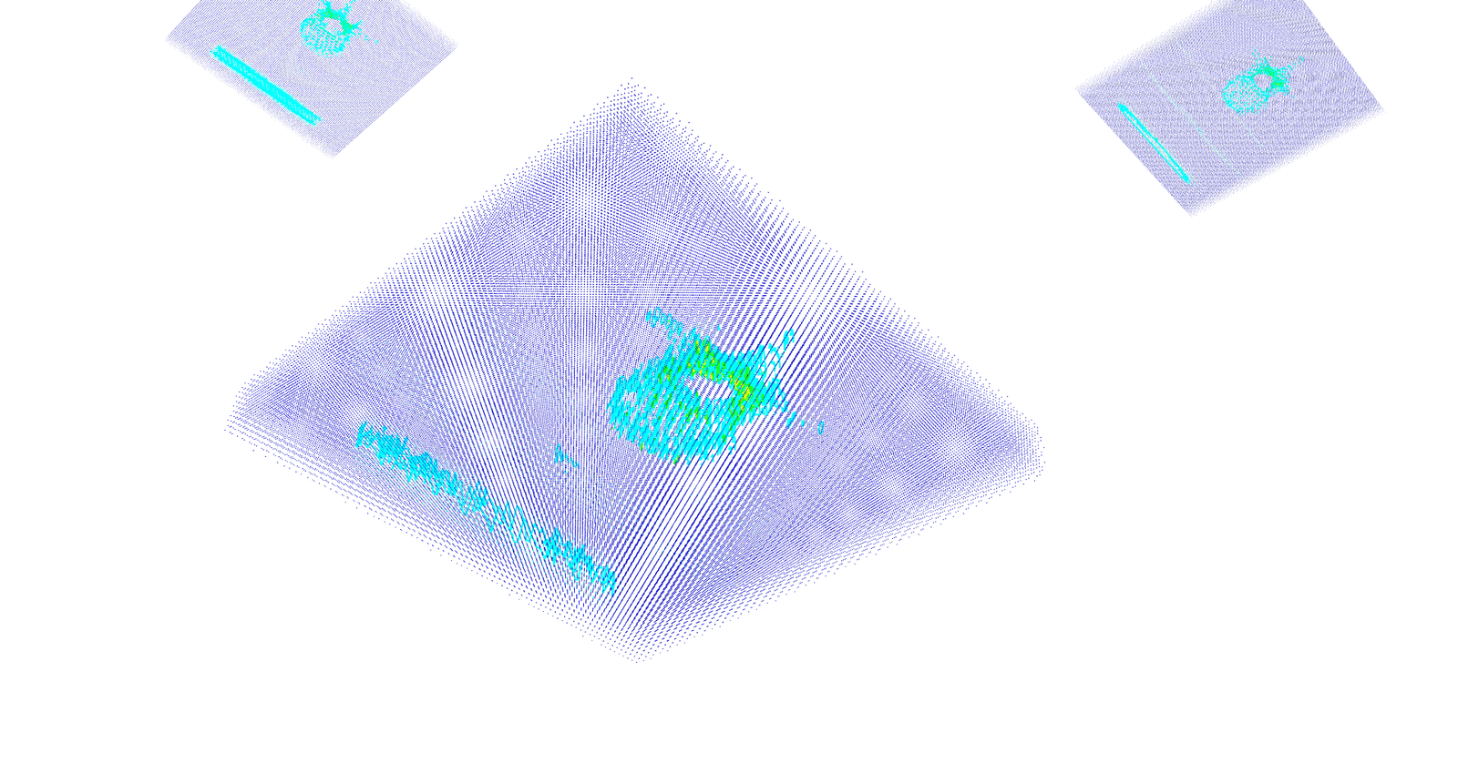
Figure 7: 3D Point Cloud of Lumbar Vertebra Using Mayavi.
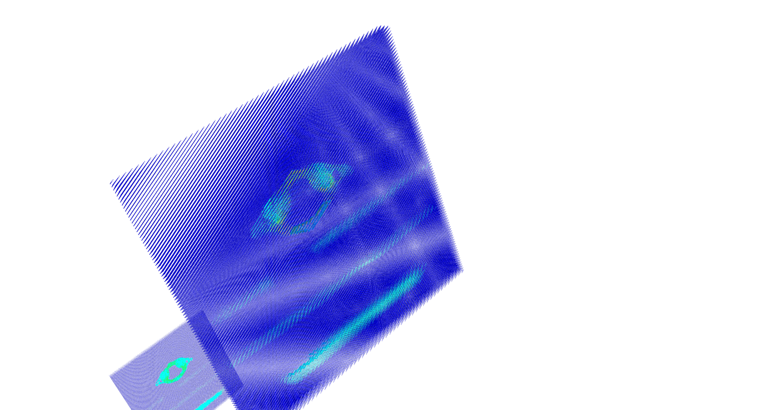
Figure 8: 3D Point Cloud of Cervical Vertebra Using Mayavi.
The point cloud thus generated as in (Figures 7 & 8) have three main issues:
i. The point clouds generated as based on equ-1 which caters for pixel spacing, however, does not cater for inter slice spacing.
ii. Owing to huge number of points (over 20 Million) processing of these points even for GPU based graphing library Mayavi is a slow process that takes considerable time.
iii. In addition to the point cloud two ghost slices are also being plotted on canvas.
The first problem is easily resolved using affine matrix of the form:
Where δt1, δt2 and δt3 are slice spacing in x,y and z axis. These are obtained from image position information available in dicom header. Listing of the code for reference:
$$ S array = np . float32 ( np . array ( image position ))$$
$$ d e l t a t 1 = S array [0][0] - S array [ len ( S array ) - 1][0]$$
$$ d e l t a t 2 = S array [1][1] - S array [ len ( S array ) - 1][1] $$
$$ d e l t a t 3 = S array [2][2] - S array [ len ( S array ) - 1][2] $$
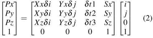
The second problem is resolved by reducing unwanted calculation on the sparse input dicom images, thereby reducing the number of pixels to be processed from 20 Million to 0.15 Million. Resulting point cloud after zero pixel removal is shown as per (Figure 9).
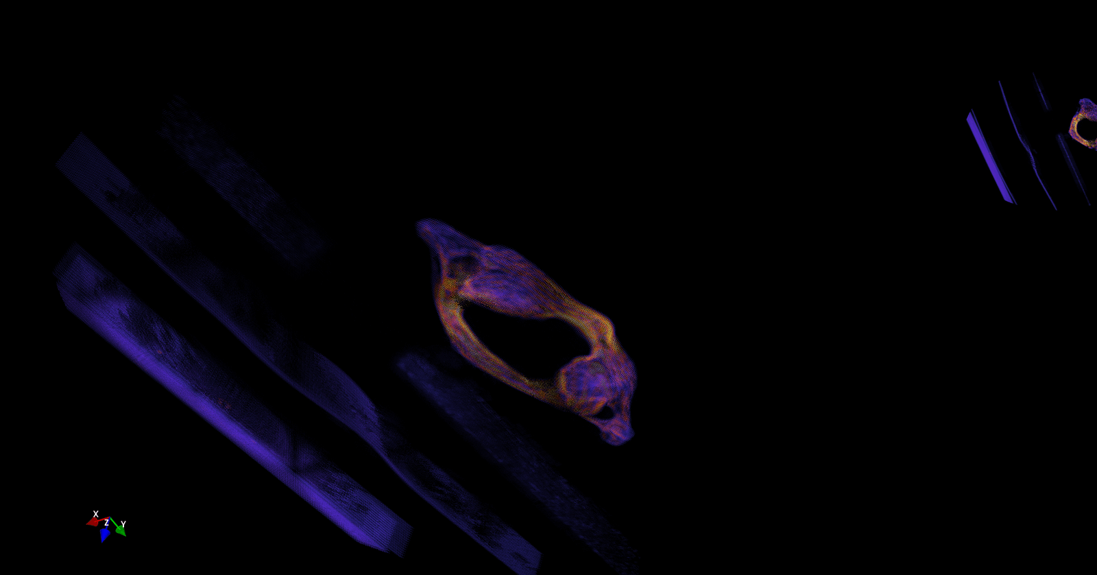
Figure 9: Point Cloud after removal of Unnecessary pixels.
However, in (Figure 9) it is obvious that apart from cervical vertebra there are ghost slices which have occurred due to artifacts in the input dicom image. Therefore, to remove these ghost slices, two approaches can be used. In the first approach, the input dicom image can be preprocessed to filter out undesired artifacts. Or, in the second approach, density-based clustering can be used.
Results
Two parameters were used for comparison i.e. Mean Square Error and Structural Similarity Index. Visualization similarity of GPU implemented cervical vertebra models using Marching Cubes and Raycasting were found comparable, however both algorithms produced about 40 percent similar results by comparing their 2D images with cervical vertebra image (Figures 10 & 11). Proposed efficient 3D reconstruction method using Affine Transform utilizing Mayavi framework and numpy matrices has produced better 3D model which is both visually appealing and computationally efficient. Same has been shown as per (Table 1).
Figure 10: Marching Cubes Similarity and MSE.
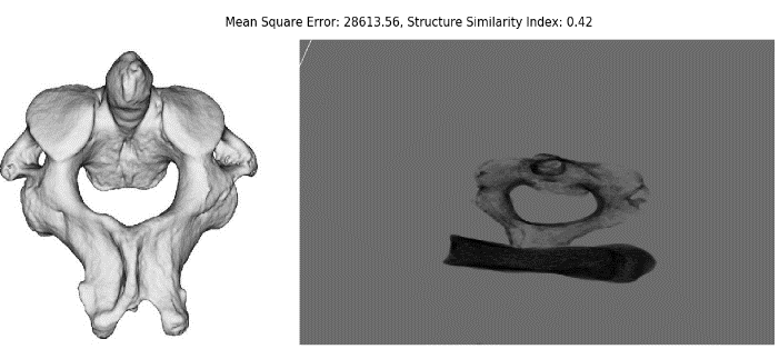
Figure 11: RayCasting Similarity and MSE.
Table 1: Performance Comparison.
|
Ser |
Algorithm |
Platform |
SSIE |
Latency |
|
1 |
Marching Cubes |
CPU |
0.38 |
300 sec |
|
2 |
Marching Cubes |
GPU |
0.43 |
2 sec |
|
3 |
RayCasting |
GPU |
0.42 |
10 sec |
|
4 |
Proposed Method |
CPU |
0.56 |
3 sec |
Future Work
We intend to follow the proposed framework (Figure 6) for developing an accurate and minimum latency model for spine vertebra. Our further work will intend to filter out ghost artifacts produced due to CT scan anomalies. These ghost slices can be removed either through filtering dicom images or clustering. We intend to use GPU accelerated clustering using pycuda gpuarrays. To improve upon the results we intend to follow the steps highlighted in red colour in figure 6 for further improvement in results. In doing so optical flow based technique for point clouds surface generation will also be explored [9].
Conflicts of Interest
None.
Article Info
Article Type
Research ArticlePublication history
Received: Sat 04, Jul 2020Accepted: Thu 16, Jul 2020
Published: Sat 25, Jul 2020
Copyright
© 2023 Usman Khan. This is an open-access article distributed under the terms of the Creative Commons Attribution License, which permits unrestricted use, distribution, and reproduction in any medium, provided the original author and source are credited. Hosting by Science Repository.DOI: 10.31487/j.MIRS.2020.01.02
Figures & Tables
Table 1: Performance Comparison.
|
Ser |
Algorithm |
Platform |
SSIE |
Latency |
|
1 |
Marching Cubes |
CPU |
0.38 |
300 sec |
|
2 |
Marching Cubes |
GPU |
0.43 |
2 sec |
|
3 |
RayCasting |
GPU |
0.42 |
10 sec |
|
4 |
Proposed Method |
CPU |
0.56 |
3 sec |
References
- Usman Khan, AmanUllah Yasin, Muhammad Abid, Imran Shafi, Shoab A Khan (2018) A Methodological Review of 3D Reconstruction Techniques in Tomographic Imaging. J Med Sys 42: 190. [Crossref]
- Turner Whitted (1980) An improved illumination model for shaded display. Communications of the ACM 23: 343-349.
- James F Blinn (1977) Models of light reflection for computer synthesized pictures. ACM SIGGRAPH Computer Graphics 11: 192-198.
- J T Kajiya (1983) New techniques for ray tracing procedurally defined objects. ACM SIGGRAPH Computer Graphics 17: 91-102.
- Marc Levoy (1990) A hybrid ray tracer for rendering polygon and volume data. IEEE Computer Graphics and Applications 10: 33-40.
- William E Lorensen, Harvey E Cline (1987) Marching cubes: A high resolution 3D surface construction algorithm. ACM SIGGRAPH Computer Graphics 21: 163-169.
- Naiwen (2019) Shaded Surface Display Technique.
- Bone CT-Scan Data (2019).
- Khan U, Klette R (2016) Logarithmically Improved Property Regression for Crowd Counting. In: Braunl T, McCane B, Rivera M, Yu X (eds) Image and Video Technology. PSIVT 2015. Lecture Notes in Computer Science, vol 9431. Springer, Cham.